Introduction
The OMOP Common Data Model
Introduction: The OMOP Common Data Model
Every time that someone goes to the doctor and something happens the doctors write it into their records.
Each annotation of the doctor is translated into a code, combination of letters and numbers that refers to a condition. There exist several different codding languages: SNOMED, read codes, ICD10, ICD9, RxNorm, ATC, … It depends on the region, language, type of record and others which one is used. This makes that the same condition or drug can be coded in different ways.
A compilation of these records for a group of people is what we call the medical databases. Depending on the origin and purpose of these data there are different groups of databases: electronic health records, claims data, registries… This databases can be structured by several different tables.
The Observational Medical Outcomes Partnership (OMOP) Common Data Model (CDM) is an open community data standard, designed to standardize the structure and content of observational data and to enable efficient analyses that can produce reliable evidence.
Standarization of the data format
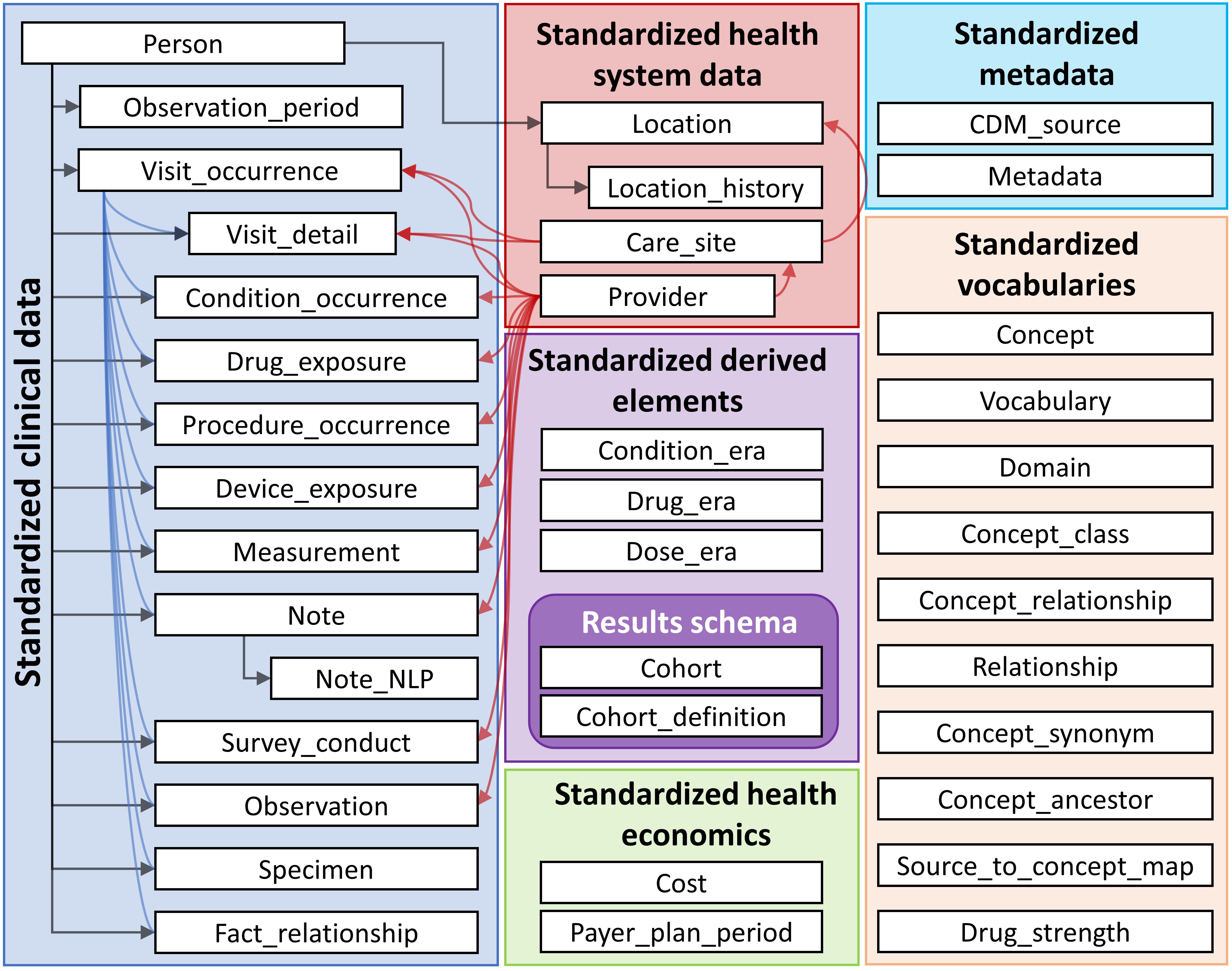
Tables and relation in the OMOP Common Data Model
Mapping a database to the OMOP CDM

Mapping process
Mapping a database to the OMOP CDM

Mapping process
Mapping a database to the OMOP CDM

Mapping process
Standarization of the vocabularies
From all the vocabularies OMOP CDM uses only a few as Standard: SNOMED for conditions, RxNorm for drugs, …
The process to obtain an standard code from non standard one is called mapping. We can find the mapping in the concept_relationship table.
Each one of the records in clinical data tables (condition_occurrence, drug_exposure, measurement, observation, …) will be coded by two codes:
Source concept: particular to each database, it is the
originalcode.Standard concept: equivalent code from the standard vocabulary.
Example of mapping
In concept relationship we can find different information such as:

Concept relationship
In particular, we have the Maps to and Mapped from relations that can help us to see the mapping between codes.
Example of mapping

Mapping process
Example of mapping

Mapping process
Example of mapping

Mapping process
More details
For more details on how the vocabularies work you can check: Vocabulary course in EHDEN academy
All details about OMOP CDM and more can be found in: the book of ohdsi.

Posit cloud

Connecting to a database from R (the DBI package)
Database connections from R can be made using the DBI package.
Connecting to a database from R (the DBI package)
Connect to Sql server:
In this CDMConnector article you can see how to connect to the different supported DBMS.
Connect to eunomia
Eunomia is a synthetic OMOP database with ~2,600 individuals. It is freely available and you can download it as:
library(CDMConnector)
library(here)
downloadEunomiaData(pathToData = here("eunomia"), overwrite = TRUE)
Download completed!Sys.setenv("EUNOMIA_DATA_FOLDER" = here("eunomia"))To connect to this database we are going to use duckdb
library(duckdb)
db <- dbConnect(duckdb(), dbdir = eunomia_dir())
db
Databases organization
Databases are organized by schemas (blueprint or plan that defines how the data will be organized and structured within the database).
In general, OMOP databases have two schemas:
cdm schema: it contains all the tables of the cdm. Usually we only will have reading permission for this schema.write schema: it is a place where we can store tables (like cohorts). We need writing permissions to this schema.
Eunomia only has a single schema (main) that will be used as cdm schema and write schema.
Read tables in Eunomia
With dbListTables we can see the tables that we can access from a connection:
dbListTables(db) [1] "care_site" "cdm_source" "concept"
[4] "concept_ancestor" "concept_class" "concept_relationship"
[7] "concept_synonym" "condition_era" "condition_occurrence"
[10] "cost" "death" "device_exposure"
[13] "domain" "dose_era" "drug_era"
[16] "drug_exposure" "drug_strength" "fact_relationship"
[19] "location" "measurement" "metadata"
[22] "note" "note_nlp" "observation"
[25] "observation_period" "payer_plan_period" "person"
[28] "procedure_occurrence" "provider" "relationship"
[31] "source_to_concept_map" "specimen" "visit_detail"
[34] "visit_occurrence" "vocabulary" Read tables in Eunomia
We can read one of this tables using dplyr:
# Source:   table<person> [?? x 18]
# Database: DuckDB 0.9.0 [martics@Windows 10 x64:R 4.2.3/C:\Users\martics\AppData\Local\Temp\RtmpGWSSC6\file6d10509a3a8a.duckdb]
   person_id gender_concept_id year_of_birth month_of_birth day_of_birth
       <int>             <int>         <int>          <int>        <int>
 1         6              8532          1963             12           31
 2       123              8507          1950              4           12
 3       129              8507          1974             10            7
 4        16              8532          1971             10           13
 5        65              8532          1967              3           31
 6        74              8532          1972              1            5
 7        42              8532          1909             11            2
 8       187              8507          1945              7           23
 9        18              8532          1965             11           17
10       111              8532          1975              5            2
# ℹ more rows
# ℹ 13 more variables: birth_datetime <dttm>, race_concept_id <int>,
#   ethnicity_concept_id <int>, location_id <int>, provider_id <int>,
#   care_site_id <int>, person_source_value <chr>, gender_source_value <chr>,
#   gender_source_concept_id <int>, race_source_value <chr>,
#   race_source_concept_id <int>, ethnicity_source_value <chr>,
#   ethnicity_source_concept_id <int>
Read tables in Eunomia
You can save the reference of this person table to a variable:
person_db <- tbl(db, "person")
person_db
# Source: table<person> [?? x 18]
# Database: DuckDB 0.9.0 [martics@Windows 10 x64:R 4.2.3/C:\Users\martics\AppData\Local\Temp\RtmpGWSSC6\file6d10509a3a8a.duckdb]
person_id gender_concept_id year_of_birth month_of_birth day_of_birth
<int> <int> <int> <int> <int>
1 6 8532 1963 12 31
2 123 8507 1950 4 12
3 129 8507 1974 10 7
4 16 8532 1971 10 13
5 65 8532 1967 3 31
6 74 8532 1972 1 5
7 42 8532 1909 11 2
8 187 8507 1945 7 23
9 18 8532 1965 11 17
10 111 8532 1975 5 2
# ℹ more rows
# ℹ 13 more variables: birth_datetime <dttm>, race_concept_id <int>,
# ethnicity_concept_id <int>, location_id <int>, provider_id <int>,
# care_site_id <int>, person_source_value <chr>, gender_source_value <chr>,
# gender_source_concept_id <int>, race_source_value <chr>,
# race_source_concept_id <int>, ethnicity_source_value <chr>,
# ethnicity_source_concept_id <int>Read tables in Eunomia
Once we read a table we can operate with it and for example count the number of rows of person table.
Read tables in Eunomia
If you are familiarized with tidyverse you can use any of the usual dplyr commands in you database tables.
tbl(db, "drug_exposure") %>%
  group_by(drug_concept_id) %>%
  summarise(number_persons = n_distinct(person_id)) %>%
  arrange(desc(number_persons))
# Source: SQL [?? x 2]
# Database: DuckDB 0.9.0 [martics@Windows 10 x64:R 4.2.3/C:\Users\martics\AppData\Local\Temp\RtmpGWSSC6\file6d10509a3a8a.duckdb]
# Ordered by: desc(number_persons)
drug_concept_id number_persons
<int> <dbl>
1 40213227 2660
2 1127433 2580
3 40213160 2140
4 1713671 2021
5 19059056 1927
6 1118084 1844
7 40213296 1737
8 40213306 1560
9 1127078 1428
10 40229134 1393
# ℹ more rowsCDMConnector

Creating a reference to the OMOP common data model
We already know what the structure of the OMOP CDM looks like. The CDMConnector package was made to help you to quickly create a reference to the OMOP CDM data as a whole.
- To install any of these packages that we use you can type:
install.packages("CDMConnector")in the console.
Creating a reference to the OMOP common data model
cdm <- cdmFromCon(con = db, cdmSchema = "main", writeSchema = "main")
cdm
# OMOP CDM reference (tbl_duckdb_connection)
Tables: person, observation_period, visit_occurrence, visit_detail, condition_occurrence, drug_exposure, procedure_occurrence, device_exposure, measurement, observation, death, note, note_nlp, specimen, fact_relationship, location, care_site, provider, payer_plan_period, cost, drug_era, dose_era, condition_era, metadata, cdm_source, concept, vocabulary, domain, concept_class, concept_relationship, relationship, concept_synonym, concept_ancestor, source_to_concept_map, drug_strengthCreating a reference to the OMOP common data model
Once we have created the our reference to the overall OMOP CDM, we can reference specific tables using the “$” operator or [[““]].
# Source: SQL [2 x 5]
# Database: DuckDB 0.9.0 [martics@Windows 10 x64:R 4.2.3/C:\Users\martics\AppData\Local\Temp\RtmpGWSSC6\file6d10509a3a8a.duckdb]
observation_period_id person_id observation_period_st…¹ observation_period_e…²
<int> <int> <date> <date>
1 6 6 1963-12-31 2007-02-06
2 13 13 2009-04-26 2019-04-14
# ℹ abbreviated names: ¹observation_period_start_date,
# ²observation_period_end_date
# ℹ 1 more variable: period_type_concept_id <int># Source: SQL [2 x 5]
# Database: DuckDB 0.9.0 [martics@Windows 10 x64:R 4.2.3/C:\Users\martics\AppData\Local\Temp\RtmpGWSSC6\file6d10509a3a8a.duckdb]
observation_period_id person_id observation_period_st…¹ observation_period_e…²
<int> <int> <date> <date>
1 6 6 1963-12-31 2007-02-06
2 13 13 2009-04-26 2019-04-14
# ℹ abbreviated names: ¹observation_period_start_date,
# ²observation_period_end_date
# ℹ 1 more variable: period_type_concept_id <int>%>% head(2) was used to only show the first 2 lines.
Creating a reference to the OMOP common data model
With this you can start playing with the tables and for example see which are the individuals with more drug_exposure records:
# Source:     SQL [?? x 2]
# Database:   DuckDB 0.9.0 [martics@Windows 10 x64:R 4.2.3/C:\Users\martics\AppData\Local\Temp\RtmpGWSSC6\file6d10509a3a8a.duckdb]
# Groups:     person_id
# Ordered by: desc(n)
   person_id     n
       <int> <dbl>
 1        36    54
 2      2333    50
 3      1478    47
 4      2985    45
 5      3708    44
 6      1746    44
 7      4297    43
 8      3695    42
 9      4613    42
10      1626    41
# ℹ more rows
Database name
When we have a cdm object we can check which is the name of that database using:
cdmName(cdm)[1] "Synthea synthetic health database"In some cases we want to give a database a name that we want, this can be done at the connection stage:
cdm <- cdmFromCon(
  con = db, cdmSchema = "main", writeSchema = "main", cdmName = "EUNOMIA"
)cdmName(cdm)[1] "EUNOMIA"Database snapshot
The database snapshot is a useful tool to get information on the characteristics of your database:
Rows: 1
Columns: 13
$ cdm_name                               <chr> "EUNOMIA"
$ cdm_source_name                        <chr> "Synthea synthetic health datab…
$ cdm_description                        <chr> "SyntheaTM is a Synthetic Patie…
$ cdm_documentation_reference            <chr> "https://synthetichealth.github…
$ cdm_version                            <chr> "v5.3.1"
$ cdm_holder                             <chr> "OHDSI Community"
$ cdm_release_date                       <chr> "2019-05-25"
$ vocabulary_version                     <chr> "v5.0 18-JAN-19"
$ person_count                           <chr> "2694"
$ observation_period_count               <chr> "5343"
$ earliest_observation_period_start_date <chr> "1908-09-22"
$ latest_observation_period_end_date     <chr> "2019-07-03"
$ snapshot_date                          <chr> "2023-10-05"
In network studies this can be very useful to export the characteristics of each one of the databases.
Generate a cohort
Let’s pick the first concept that we see in condition_occurrence to build a cohort:
cdm$condition_occurrence# Source: table<main.condition_occurrence> [?? x 16]
# Database: DuckDB 0.9.0 [martics@Windows 10 x64:R 4.2.3/C:\Users\martics\AppData\Local\Temp\RtmpGWSSC6\file6d10509a3a8a.duckdb]
condition_occurrence_id person_id condition_concept_id condition_start_date
<int> <int> <int> <date>
1 4483 263 4112343 2015-10-02
2 4657 273 192671 2011-10-10
3 4815 283 28060 1984-02-15
4 4981 293 378001 2005-11-07
5 5153 304 257012 1974-07-30
6 5313 312 4134304 1991-05-14
7 5513 326 28060 1979-09-23
8 5655 334 40481087 1999-07-12
9 5811 341 40481087 1990-09-14
10 5977 351 40481087 1986-02-24
# ℹ more rows
# ℹ 12 more variables: condition_start_datetime <dttm>,
# condition_end_date <date>, condition_end_datetime <dttm>,
# condition_type_concept_id <int>, condition_status_concept_id <int>,
# stop_reason <chr>, provider_id <int>, visit_occurrence_id <int>,
# visit_detail_id <int>, condition_source_value <chr>,
# condition_source_concept_id <int>, condition_status_source_value <chr># Source: SQL [1 x 10]
# Database: DuckDB 0.9.0 [martics@Windows 10 x64:R 4.2.3/C:\Users\martics\AppData\Local\Temp\RtmpGWSSC6\file6d10509a3a8a.duckdb]
concept_id concept_name domain_id vocabulary_id concept_class_id
<int> <chr> <chr> <chr> <chr>
1 4112343 Acute viral pharyngitis Condition SNOMED Clinical Finding
# ℹ 5 more variables: standard_concept <chr>, concept_code <chr>,
# valid_start_date <date>, valid_end_date <date>, invalid_reason <chr>Generate a cohort
We can instantiate this cohort using the function: generateConceptCohortSet
cdm <- generateConceptCohortSet(
  cdm = cdm,
  name = "my_first_cohort",
  conceptSet = list("acute_viral_pharyngitis" = 4112343),
  end = "event_end_date",
  limit = "all",
  overwrite = TRUE
)

cdm$my_first_cohort
# Source: table<main.my_first_cohort> [?? x 4]
# Database: DuckDB 0.9.0 [martics@Windows 10 x64:R 4.2.3/C:\Users\martics\AppData\Local\Temp\RtmpGWSSC6\file6d10509a3a8a.duckdb]
cohort_definition_id subject_id cohort_start_date cohort_end_date
<int> <int> <date> <date>
1 1 57 1983-12-03 1983-12-10
2 1 187 1978-11-05 1978-11-16
3 1 187 1996-04-08 1996-04-19
4 1 211 1972-11-16 1972-11-29
5 1 222 1967-01-19 1967-01-30
6 1 248 2013-01-16 2013-01-24
7 1 390 1977-03-29 1977-04-05
8 1 394 1955-02-10 1955-02-18
9 1 394 1978-08-11 1978-08-24
10 1 502 2016-10-15 2016-10-24
# ℹ more rowsGenerate a cohort
# Source:   SQL [6 x 4]
# Database: DuckDB 0.9.0 [martics@Windows 10 x64:R 4.2.3/C:\Users\martics\AppData\Local\Temp\RtmpGWSSC6\file6d10509a3a8a.duckdb]
  cohort_definition_id subject_id cohort_start_date cohort_end_date
                 <int>      <int> <date>            <date>
1                    1        263 1960-10-20        1960-10-30
2                    1        263 1997-08-01        1997-08-12
3                    1        263 2015-10-02        2015-10-14
4                    1        263 1991-04-25        1991-05-03
5                    1        263 2014-07-28        2014-08-05
6                    1        263 2002-12-16        2002-12-24
Generate a cohort
Once we instantiate a cohort the cohort is in a permanent table in the database, which means that if I disconnect from the database and connect again the cohort will still be there.
We can read existing cohorts in the database with the argument cohortTables when creating the connection.
Read an existing cohort
You can read an existing cohort when you create the cdm object
cdm <- cdmFromCon(
  con = db, cdmSchema = "main", writeSchema = "main", cohortTables = c("my_first_cohort")
)
cdm$my_first_cohort
# Source: table<main.my_first_cohort> [?? x 4]
# Database: DuckDB 0.9.0 [martics@Windows 10 x64:R 4.2.3/C:\Users\martics\AppData\Local\Temp\RtmpGWSSC6\file6d10509a3a8a.duckdb]
cohort_definition_id subject_id cohort_start_date cohort_end_date
<int> <int> <date> <date>
1 1 57 1983-12-03 1983-12-10
2 1 187 1978-11-05 1978-11-16
3 1 187 1996-04-08 1996-04-19
4 1 211 1972-11-16 1972-11-29
5 1 222 1967-01-19 1967-01-30
6 1 248 2013-01-16 2013-01-24
7 1 390 1977-03-29 1977-04-05
8 1 394 1955-02-10 1955-02-18
9 1 394 1978-08-11 1978-08-24
10 1 502 2016-10-15 2016-10-24
# ℹ more rowsExploring concept cohort creation
Let’s create a cohort of paracetamol and diclofenac records.
library(CodelistGenerator)
codelist <- getDrugIngredientCodes(cdm, c("acetaminophen", "diclofenac"))
cdm <- generateConceptCohortSet(
cdm = cdm, conceptSet = codelist, name = "drugs_obs", limit = "all", end = "observation_period_end_date"
)cdm$drugs_obs# Source: table<main.drugs_obs> [?? x 4]
# Database: DuckDB 0.9.0 [martics@Windows 10 x64:R 4.2.3/C:\Users\martics\AppData\Local\Temp\RtmpGWSSC6\file6d10509a3a8a.duckdb]
cohort_definition_id subject_id cohort_start_date cohort_end_date
<int> <int> <date> <date>
1 1 19 1985-05-16 2018-08-19
2 1 1634 1978-12-18 2018-09-21
3 1 2326 1994-01-13 2019-05-23
4 1 2933 1998-07-30 2018-11-19
5 1 3221 2000-06-11 2018-06-30
6 1 3389 1996-06-08 2018-10-29
7 1 3579 1997-09-08 2018-11-24
8 1 4121 1964-10-19 1987-11-15
9 1 4160 2004-08-08 2018-07-13
10 2 86 1952-04-03 2019-06-04
# ℹ more rowsExploring concept cohort creation
cdm <- generateConceptCohortSet(
  cdm = cdm, conceptSet = codelist, name = "drugs_event", limit = "all", end = "event_end_date"
)cdm$drugs_event# Source: table<main.drugs_event> [?? x 4]
# Database: DuckDB 0.9.0 [martics@Windows 10 x64:R 4.2.3/C:\Users\martics\AppData\Local\Temp\RtmpGWSSC6\file6d10509a3a8a.duckdb]
cohort_definition_id subject_id cohort_start_date cohort_end_date
<int> <int> <date> <date>
1 1 488 1993-12-10 1993-12-10
2 1 954 2015-12-15 2015-12-15
3 1 2218 2011-08-03 2011-08-03
4 1 3090 2001-02-02 2001-02-02
5 2 12 1964-08-22 1964-09-05
6 2 36 2001-03-30 2001-03-30
7 2 116 1959-07-22 1959-08-12
8 2 186 1991-01-11 1991-01-25
9 2 316 1956-11-04 1956-11-18
10 2 316 2012-02-01 2012-05-01
# ℹ more rowsCohort attributes
Cohorts has a new class called ‘GeneratedCohortSet’:
class(cdm$my_first_cohort)This allows us to get some extra information from this objects a part from the list of individuals in the cohort:
cohort set: equivalence between cohort_definition_id and the cohort name or parameters used in each cohort (
cohortSet).cohort counts: number of subjects and records per cohort (
cohortCount).cohort attrition: attrition of the different cohorts (
cohortAttrition).
Cohort set
cohortSet(cdm$drugs_obs)# A tibble: 2 × 2
cohort_definition_id cohort_name
<int> <chr>
1 1 Ingredient: Diclofenac (1124300)
2 2 Ingredient: Acetaminophen (1125315)cohortSet(cdm$drugs_event)# A tibble: 2 × 2
cohort_definition_id cohort_name
<int> <chr>
1 1 Ingredient: Diclofenac (1124300)
2 2 Ingredient: Acetaminophen (1125315)Cohort count
cohortCount(cdm$drugs_obs)# A tibble: 2 × 3
cohort_definition_id number_records number_subjects
<int> <dbl> <dbl>
1 1 830 830
2 2 2679 2679cohortCount(cdm$drugs_event)# A tibble: 2 × 3
cohort_definition_id number_records number_subjects
<int> <dbl> <dbl>
1 1 830 830
2 2 13908 2679Cohort attrition
cohortAttrition(cdm$drugs_obs)# A tibble: 2 × 7
cohort_definition_id number_records number_subjects reason_id reason
<int> <dbl> <dbl> <dbl> <chr>
1 1 830 830 1 Qualifying init…
2 2 2679 2679 1 Qualifying init…
# ℹ 2 more variables: excluded_records <dbl>, excluded_subjects <dbl>cohortAttrition(cdm$drugs_event)# A tibble: 2 × 7
cohort_definition_id number_records number_subjects reason_id reason
<int> <dbl> <dbl> <dbl> <chr>
1 1 830 830 1 Qualifying init…
2 2 13908 2679 1 Qualifying init…
# ℹ 2 more variables: excluded_records <dbl>, excluded_subjects <dbl>Add a new line to the attrition table
cdm$drugs_event <- cdm$drugs_event %>%
  group_by(cohort_definition_id, subject_id) %>%
  filter(cohort_start_date == min(cohort_start_date, na.rm = TRUE)) %>%
  ungroup() %>%
  computeQuery() %>%
  recordCohortAttrition("limit to first observation")

cohortAttrition(cdm$drugs_event)
# A tibble: 4 × 7
cohort_definition_id number_records number_subjects reason_id reason
<int> <dbl> <dbl> <dbl> <chr>
1 1 830 830 1 Qualifying init…
2 1 830 830 2 limit to first …
3 2 13908 2679 1 Qualifying init…
4 2 2679 2679 2 limit to first …
# ℹ 2 more variables: excluded_records <dbl>, excluded_subjects <dbl>IncidencePrevalence

Oveview
- Concepts
- Development
- Interface
Concepts
Denominator population
Incidence rates
-
Prevalence
Point prevalence
Period prevalence
Denominator population
Observation periods
(4)-denominator%20no%20criteria.drawio.png)
Denominator population
Observation periods + study period
(4)-denom%20study%20period.drawio.png)
Denominator population
Observation periods + study period + prior history requirement
(4)-denom%20without%20age.drawio-01.png)
Denominator population
Observation periods + study period + prior history requirement + age (and sex) restriction

Incidence rates
Washout all history, no repetitive events

Incidence rates
No washout, no repetitive events

Incidence rates
Some washout, no repetitive events

Incidence rates
Some washout, repetitive events

Prevalence
Point prevalence

Prevalence
Period prevalence

Oveview
- Concepts
- Development
- Interface
Face validity

Software performance

Dissemination

Oveview
- Concepts
- Development
- Interface
Required packages
install.packages("IncidencePrevalence")generateDenominatorCohortSet()
cdm <- mockIncidencePrevalenceRef(sampleSize = 5000)

cdm <- generateDenominatorCohortSet(cdm, name = "dpop")

cdm$dpop %>%
  glimpse()
Rows: ??
Columns: 4
Database: DuckDB 0.9.0 [martics@Windows 10 x64:R 4.2.3/:memory:]
$ cohort_definition_id <int> 1, 1, 1, 1, 1, 1, 1, 1, 1, 1, 1, 1, 1, 1, 1, 1, 1…
$ subject_id <chr> "1", "2", "3", "4", "5", "6", "7", "8", "9", "10"…
$ cohort_start_date <date> 2013-12-18, 2018-05-09, 2006-05-07, 2010-08-25, …
$ cohort_end_date <date> 2014-12-30, 2019-05-16, 2007-02-02, 2011-02-12, …generateDenominatorCohortSet()
cdm <- generateDenominatorCohortSet(
  cdm = cdm,
  name = "dpop",
  cohortDateRange = c(as.Date("2008-01-01"),
                      as.Date("2012-01-01"))
)
cdm$dpop %>%
  glimpse()
Rows: ??
Columns: 4
Database: DuckDB 0.9.0 [martics@Windows 10 x64:R 4.2.3/:memory:]
$ cohort_definition_id <int> 1, 1, 1, 1, 1, 1, 1, 1, 1, 1, 1, 1, 1, 1, 1, 1, 1…
$ subject_id <chr> "4", "7", "8", "11", "12", "14", "15", "16", "19"…
$ cohort_start_date <date> 2010-08-25, 2009-02-19, 2008-09-01, 2008-12-18, …
$ cohort_end_date <date> 2011-02-12, 2011-06-10, 2008-10-15, 2010-08-13, …generateDenominatorCohortSet()
cdm <- generateDenominatorCohortSet(
  cdm = cdm,
  name = "dpop",
  cohortDateRange = c(as.Date("2008-01-01"),
                      as.Date("2012-01-01")),
  ageGroup = list(
    c(0, 49),
    c(50, 100)
  ),
  sex = c("Male", "Female")
)

cdm$dpop %>%
  glimpse()
Rows: ??
Columns: 4
Database: DuckDB 0.9.0 [martics@Windows 10 x64:R 4.2.3/:memory:]
$ cohort_definition_id <int> 1, 1, 1, 1, 1, 1, 1, 1, 1, 1, 1, 1, 1, 1, 1, 1, 1…
$ subject_id <chr> "4", "14", "15", "25", "26", "31", "46", "55", "7…
$ cohort_start_date <date> 2010-08-25, 2009-10-19, 2011-10-23, 2009-07-09, …
$ cohort_end_date <date> 2011-02-12, 2010-11-27, 2012-01-01, 2010-02-11, …generateDenominatorCohortSet()
cdm <- generateDenominatorCohortSet(
  cdm = cdm, name = "dpop",
  cohortDateRange = c(as.Date("2008-01-01"),
                      endDate = as.Date("2012-01-01")),
  ageGroup = list(
    c(0, 49),
    c(50, 100)
  ),
  sex = c("Male", "Female", "Both"),
  daysPriorHistory = c(0, 180)
)

cdm$dpop %>%
  glimpse()
Rows: ??
Columns: 4
Database: DuckDB 0.9.0 [martics@Windows 10 x64:R 4.2.3/:memory:]
$ cohort_definition_id <int> 1, 1, 1, 1, 1, 1, 1, 1, 1, 1, 1, 1, 1, 1, 1, 1, 1…
$ subject_id <chr> "4", "14", "15", "25", "26", "31", "46", "55", "7…
$ cohort_start_date <date> 2010-08-25, 2009-10-19, 2011-10-23, 2009-07-09, …
$ cohort_end_date <date> 2011-02-12, 2010-11-27, 2012-01-01, 2010-02-11, …generateDenominatorCohortSet()
cohortSet(cdm$dpop)# A tibble: 12 × 10
cohort_definition_id cohort_name age_group sex days_prior_history
<int> <chr> <chr> <chr> <dbl>
1 1 Denominator cohort 1 0 to 49 Male 0
2 2 Denominator cohort 2 0 to 49 Male 180
3 3 Denominator cohort 3 0 to 49 Fema… 0
4 4 Denominator cohort 4 0 to 49 Fema… 180
5 5 Denominator cohort 5 0 to 49 Both 0
6 6 Denominator cohort 6 0 to 49 Both 180
7 7 Denominator cohort 7 50 to 100 Male 0
8 8 Denominator cohort 8 50 to 100 Male 180
9 9 Denominator cohort 9 50 to 100 Fema… 0
10 10 Denominator cohort 10 50 to 100 Fema… 180
11 11 Denominator cohort 11 50 to 100 Both 0
12 12 Denominator cohort 12 50 to 100 Both 180
# ℹ 5 more variables: start_date <date>, end_date <date>,
# strata_cohort_definition_id <lgl>, strata_cohort_name <lgl>,
# closed_cohort <lgl>generateDenominatorCohortSet()
cohortCount(cdm$dpop)# A tibble: 12 × 3
cohort_definition_id number_records number_subjects
<int> <dbl> <dbl>
1 1 488 488
2 2 367 367
3 3 461 461
4 4 355 355
5 5 949 949
6 6 722 722
7 7 450 450
8 8 360 360
9 9 463 463
10 10 370 370
11 11 913 913
12 12 730 730generateDenominatorCohortSet()
cohortAttrition(cdm$dpop) %>%
  filter(cohort_definition_id == 1)
# A tibble: 9 × 7
cohort_definition_id number_records number_subjects reason_id reason
<int> <dbl> <dbl> <dbl> <glue>
1 1 5000 5000 1 Starting popula…
2 1 5000 5000 2 Missing year of…
3 1 5000 5000 3 Missing sex
4 1 5000 5000 4 Cannot satisfy …
5 1 1836 1836 5 No observation …
6 1 1836 1836 6 Doesn't satisfy…
7 1 1836 1836 7 Prior history r…
8 1 925 925 8 Not Male
9 1 488 488 10 No observation …
# ℹ 2 more variables: excluded_records <dbl>, excluded_subjects <dbl>generateDenominatorCohortSet()
dpop <- cdm$dpop %>%
  collect() %>%
  left_join(cohortSet(cdm$dpop),
            by = "cohort_definition_id") %>%
  mutate(cohort_definition_id=as.character(cohort_definition_id))

plot <- dpop %>%
  filter(subject_id %in% c("1791", "2018", "2076", "2123")) %>%
  pivot_longer(cols = c(
    "cohort_start_date",
    "cohort_end_date"
  )) %>%
  ggplot(aes(x = subject_id, y = value, colour = cohort_definition_id)) +
  facet_grid(sex + days_prior_history ~ ., space = "free_y") +
  geom_point(position = position_dodge(width = 0.5)) +
  geom_line(position = position_dodge(width = 0.5)) +
  theme_bw() +
  theme(legend.position = "top") +
  ylab("Year") +
  coord_flip()
generateDenominatorCohortSet()
plot 
estimateIncidence()
cdm <- mockIncidencePrevalenceRef(
  sampleSize = 50000,
  outPre = 0.5
)

cdm <- generateDenominatorCohortSet(
  cdm = cdm, name = "denominator",
  cohortDateRange = c(as.Date("2008-01-01"),
                      as.Date("2012-01-01")),
  ageGroup = list(
    c(0, 17),
    c(18, 44),
    c(45, 65),
    c(66, 100)
  )
)
inc <- estimateIncidence(
  cdm = cdm,
  denominatorTable = "denominator",
  outcomeTable = "outcome",
  interval = "years",
  outcomeWashout = NULL,
  repeatedEvents = FALSE
)
estimateIncidence()
Rows: 16
Columns: 29
$ analysis_id <chr> "1", "1", "1", "1", "2", "2", …
$ n_persons <int> 814, 754, 675, 589, 2353, 2285…
$ person_days <dbl> 142280, 137134, 128548, 105016…
$ n_events <int> 192, 164, 152, 146, 571, 574, …
$ incidence_start_date <date> 2008-01-01, 2009-01-01, 2010-…
$ incidence_end_date <date> 2008-12-31, 2009-12-31, 2010-…
$ person_years <dbl> 389.5414, 375.4524, 351.9452, …
$ incidence_100000_pys <dbl> 49288.73, 43680.63, 43188.54, …
$ incidence_100000_pys_95CI_lower <dbl> 42563.16, 37251.15, 36595.63, …
$ incidence_100000_pys_95CI_upper <dbl> 56775.25, 50901.14, 50626.12, …
$ cohort_obscured <chr> "FALSE", "FALSE", "FALSE", "FA…
$ result_obscured <chr> "FALSE", "FALSE", "FALSE", "FA…
$ outcome_cohort_id <chr> "1", "1", "1", "1", "1", "1", …
$ outcome_cohort_name <chr> "cohort_1", "cohort_1", "cohor…
$ analysis_repeated_events <lgl> FALSE, FALSE, FALSE, FALSE, FA…
$ analysis_interval <chr> "years", "years", "years", "ye…
$ analysis_complete_database_intervals <lgl> TRUE, TRUE, TRUE, TRUE, TRUE, …
$ denominator_cohort_id <int> 1, 1, 1, 1, 2, 2, 2, 2, 3, 3, …
$ analysis_min_cell_count <dbl> 5, 5, 5, 5, 5, 5, 5, 5, 5, 5, …
$ denominator_cohort_name <chr> "Denominator cohort 1", "Denom…
$ denominator_age_group <chr> "0 to 17", "0 to 17", "0 to 17…
$ denominator_sex <chr> "Both", "Both", "Both", "Both"…
$ denominator_days_prior_history <dbl> 0, 0, 0, 0, 0, 0, 0, 0, 0, 0, …
$ denominator_start_date <date> 2008-01-01, 2008-01-01, 2008-…
$ denominator_end_date <date> 2012-01-01, 2012-01-01, 2012-…
$ denominator_strata_cohort_definition_id <lgl> NA, NA, NA, NA, NA, NA, NA, NA…
$ denominator_strata_cohort_name <lgl> NA, NA, NA, NA, NA, NA, NA, NA…
$ denominator_closed_cohort <lgl> FALSE, FALSE, FALSE, FALSE, FA…
$ cdm_name <chr> "test_database", "test_databas…estimateIncidence()
inc <- estimateIncidence(
cdm = cdm,
denominatorTable = "denominator",
outcomeTable = "outcome",
interval = c("Months"),
outcomeWashout = c(0, 365),
repeatedEvents = FALSE
)
inc %>%
  glimpse()
Rows: 384
Columns: 30
$ analysis_id <chr> "1", "1", "1", "1", "1", "1", …
$ n_persons <int> 582, 551, 535, 518, 495, 481, …
$ person_days <dbl> 16727, 14898, 15184, 13899, 13…
$ n_events <int> 16, 19, 17, 23, 21, 16, 12, 20…
$ incidence_start_date <date> 2008-01-01, 2008-02-01, 2008-…
$ incidence_end_date <date> 2008-01-31, 2008-02-29, 2008-…
$ person_years <dbl> 45.79603, 40.78850, 41.57153, …
$ incidence_100000_pys <dbl> 34937.53, 46581.76, 40893.37, …
$ incidence_100000_pys_95CI_lower <dbl> 19969.815, 28045.260, 23821.89…
$ incidence_100000_pys_95CI_upper <dbl> 56736.35, 72743.18, 65474.25, …
$ cohort_obscured <chr> "FALSE", "FALSE", "FALSE", "FA…
$ result_obscured <chr> "FALSE", "FALSE", "FALSE", "FA…
$ outcome_cohort_id <chr> "1", "1", "1", "1", "1", "1", …
$ outcome_cohort_name <chr> "cohort_1", "cohort_1", "cohor…
$ analysis_outcome_washout <dbl> 0, 0, 0, 0, 0, 0, 0, 0, 0, 0, …
$ analysis_repeated_events <lgl> FALSE, FALSE, FALSE, FALSE, FA…
$ analysis_interval <chr> "months", "months", "months", …
$ analysis_complete_database_intervals <lgl> TRUE, TRUE, TRUE, TRUE, TRUE, …
$ denominator_cohort_id <int> 1, 1, 1, 1, 1, 1, 1, 1, 1, 1, …
$ analysis_min_cell_count <dbl> 5, 5, 5, 5, 5, 5, 5, 5, 5, 5, …
$ denominator_cohort_name <chr> "Denominator cohort 1", "Denom…
$ denominator_age_group <chr> "0 to 17", "0 to 17", "0 to 17…
$ denominator_sex <chr> "Both", "Both", "Both", "Both"…
$ denominator_days_prior_history <dbl> 0, 0, 0, 0, 0, 0, 0, 0, 0, 0, …
$ denominator_start_date <date> 2008-01-01, 2008-01-01, 2008-…
$ denominator_end_date <date> 2012-01-01, 2012-01-01, 2012-…
$ denominator_strata_cohort_definition_id <lgl> NA, NA, NA, NA, NA, NA, NA, NA…
$ denominator_strata_cohort_name <lgl> NA, NA, NA, NA, NA, NA, NA, NA…
$ denominator_closed_cohort <lgl> FALSE, FALSE, FALSE, FALSE, FA…
$ cdm_name <chr> "test_database", "test_databas…estimateIncidence()
plotIncidence(inc, facet = "denominator_age_group")
estimatePointPrevalence() and estimatePeriodPrevalence()
cdm <- mockIncidencePrevalenceRef(
  sampleSize = 50000,
  outPre = 0.5
)

cdm <- generateDenominatorCohortSet(
  cdm = cdm, name = "denominator",
  cohortDateRange = c(as.Date("2008-01-01"),
                      as.Date("2012-01-01")),
  ageGroup = list(
    c(0, 17),
    c(18, 44),
    c(45, 65),
    c(66, 100)
  )
)
prev <- estimatePointPrevalence(
  cdm = cdm,
  denominatorTable = "denominator",
  outcomeTable = "outcome",
  interval = "Years"
)
estimatePointPrevalence() and estimatePeriodPrevalence()
Rows: 20
Columns: 30
$ analysis_id <chr> "1", "1", "1", "1", "1", "2", …
$ prevalence_start_date <date> 2008-01-01, 2009-01-01, 2010-…
$ prevalence_end_date <date> 2008-01-01, 2009-01-01, 2010-…
$ n_cases <int> NA, NA, NA, NA, 5, 5, 15, 12, …
$ n_population <int> 545, 503, 476, 407, 352, 1492,…
$ prevalence <dbl> NA, NA, NA, NA, 0.014204545, 0…
$ prevalence_95CI_lower <dbl> NA, NA, NA, NA, 0.006082190, 0…
$ prevalence_95CI_upper <dbl> NA, NA, NA, NA, 0.032815635, 0…
$ cohort_obscured <chr> "FALSE", "FALSE", "FALSE", "FA…
$ result_obscured <chr> "TRUE", "TRUE", "TRUE", "TRUE"…
$ outcome_cohort_id <chr> "1", "1", "1", "1", "1", "1", …
$ outcome_cohort_name <chr> "cohort_1", "cohort_1", "cohor…
$ analysis_outcome_lookback_days <dbl> 0, 0, 0, 0, 0, 0, 0, 0, 0, 0, …
$ analysis_type <chr> "point", "point", "point", "po…
$ analysis_interval <chr> "years", "years", "years", "ye…
$ analysis_complete_database_intervals <lgl> FALSE, FALSE, FALSE, FALSE, FA…
$ analysis_time_point <chr> "start", "start", "start", "st…
$ analysis_full_contribution <lgl> FALSE, FALSE, FALSE, FALSE, FA…
$ analysis_min_cell_count <dbl> 5, 5, 5, 5, 5, 5, 5, 5, 5, 5, …
$ denominator_cohort_id <int> 1, 1, 1, 1, 1, 2, 2, 2, 2, 2, …
$ denominator_cohort_name <chr> "Denominator cohort 1", "Denom…
$ denominator_age_group <chr> "0 to 17", "0 to 17", "0 to 17…
$ denominator_sex <chr> "Both", "Both", "Both", "Both"…
$ denominator_days_prior_history <dbl> 0, 0, 0, 0, 0, 0, 0, 0, 0, 0, …
$ denominator_start_date <date> 2008-01-01, 2008-01-01, 2008-…
$ denominator_end_date <date> 2012-01-01, 2012-01-01, 2012-…
$ denominator_strata_cohort_definition_id <lgl> NA, NA, NA, NA, NA, NA, NA, NA…
$ denominator_strata_cohort_name <lgl> NA, NA, NA, NA, NA, NA, NA, NA…
$ denominator_closed_cohort <lgl> FALSE, FALSE, FALSE, FALSE, FA…
$ cdm_name <chr> "test_database", "test_databas…estimatePointPrevalence() and estimatePeriodPrevalence()
prev <- estimatePeriodPrevalence(
cdm = cdm,
denominatorTable = "denominator",
outcomeTable = "outcome",
interval = "months"
)
prev %>%
  glimpse()
Rows: 192
Columns: 30
$ analysis_id <chr> "1", "1", "1", "1", "1", "1", …
$ prevalence_start_date <date> 2008-01-01, 2008-02-01, 2008-…
$ prevalence_end_date <date> 2008-01-31, 2008-02-29, 2008-…
$ n_cases <int> 19, 20, 20, 25, 24, 20, 17, 24…
$ n_population <int> 582, 566, 566, 557, 549, 543, …
$ prevalence <dbl> 0.03264605, 0.03533569, 0.0353…
$ prevalence_95CI_lower <dbl> 0.020997700, 0.022989020, 0.02…
$ prevalence_95CI_upper <dbl> 0.05042343, 0.05394722, 0.0539…
$ cohort_obscured <chr> "FALSE", "FALSE", "FALSE", "FA…
$ result_obscured <chr> "FALSE", "FALSE", "FALSE", "FA…
$ outcome_cohort_id <chr> "1", "1", "1", "1", "1", "1", …
$ outcome_cohort_name <chr> "cohort_1", "cohort_1", "cohor…
$ analysis_outcome_lookback_days <dbl> 0, 0, 0, 0, 0, 0, 0, 0, 0, 0, …
$ analysis_type <chr> "period", "period", "period", …
$ analysis_interval <chr> "months", "months", "months", …
$ analysis_complete_database_intervals <lgl> TRUE, TRUE, TRUE, TRUE, TRUE, …
$ analysis_time_point <chr> "start", "start", "start", "st…
$ analysis_full_contribution <lgl> FALSE, FALSE, FALSE, FALSE, FA…
$ analysis_min_cell_count <dbl> 5, 5, 5, 5, 5, 5, 5, 5, 5, 5, …
$ denominator_cohort_id <int> 1, 1, 1, 1, 1, 1, 1, 1, 1, 1, …
$ denominator_cohort_name <chr> "Denominator cohort 1", "Denom…
$ denominator_age_group <chr> "0 to 17", "0 to 17", "0 to 17…
$ denominator_sex <chr> "Both", "Both", "Both", "Both"…
$ denominator_days_prior_history <dbl> 0, 0, 0, 0, 0, 0, 0, 0, 0, 0, …
$ denominator_start_date <date> 2008-01-01, 2008-01-01, 2008-…
$ denominator_end_date <date> 2012-01-01, 2012-01-01, 2012-…
$ denominator_strata_cohort_definition_id <lgl> NA, NA, NA, NA, NA, NA, NA, NA…
$ denominator_strata_cohort_name <lgl> NA, NA, NA, NA, NA, NA, NA, NA…
$ denominator_closed_cohort <lgl> FALSE, FALSE, FALSE, FALSE, FA…
$ cdm_name <chr> "test_database", "test_databas…Your turn
Using Eunomia data:
Generate a denominator cohort (between 1st January 2000 to 1st January 2020) using
IncidencePrevalence::generateDenominatorCohortSetGet codes for diclofenac using
CodelistGenerator::getDrugIngredientCodesCreate an outcome of diclofenac using
CDMConnector::generateConceptCohortSetEstimate yearly incidence with
estimateIncidenceand yearly period prevalence withestimatePeriodPrevalenceExtend analysis to include stratification by age groups and sex
Extend analysis to include sensitivity analysis with a year of history required
Your turn
