install.packages("dplyr")
install.packages("ggplot2")
install.packages("DBI")
install.packages("duckdb")
install.packages("palmerpenguins")1 Getting started
1.1 A first data analysis in R with a database
Artwork by @allison_horst
Before we start thinking about working with health care data spread across a database using the OMOP common data model, let’s first do a quick data analysis from R using a simpler dataset held in a database to quickly understand the general approach. For this we’ll use data from palmerpenguins package, which contains data on penguins collected from the Palmer Station in Antarctica.
1.2 Getting set up
Assuming that you have R and RStudio already set up, first we need to install a few packages not included in base R if we don´t already have them.
Once installed, we can load them like so.
library(dplyr)
library(ggplot2)
library(DBI)
library(duckdb)
library(palmerpenguins)
1.3 Taking a peek at the data
We can get an overview of the data using the glimpse() command.
glimpse(penguins)Rows: 344
Columns: 8
$ species <fct> Adelie, Adelie, Adelie, Adelie, Adelie, Adelie, Adel…
$ island <fct> Torgersen, Torgersen, Torgersen, Torgersen, Torgerse…
$ bill_length_mm <dbl> 39.1, 39.5, 40.3, NA, 36.7, 39.3, 38.9, 39.2, 34.1, …
$ bill_depth_mm <dbl> 18.7, 17.4, 18.0, NA, 19.3, 20.6, 17.8, 19.6, 18.1, …
$ flipper_length_mm <int> 181, 186, 195, NA, 193, 190, 181, 195, 193, 190, 186…
$ body_mass_g <int> 3750, 3800, 3250, NA, 3450, 3650, 3625, 4675, 3475, …
$ sex <fct> male, female, female, NA, female, male, female, male…
$ year <int> 2007, 2007, 2007, 2007, 2007, 2007, 2007, 2007, 2007…Or we could take a look at the first rows of the data using head()
head(penguins, 5)# A tibble: 5 × 8
species island bill_length_mm bill_depth_mm flipper_length_mm body_mass_g
<fct> <fct> <dbl> <dbl> <int> <int>
1 Adelie Torgersen 39.1 18.7 181 3750
2 Adelie Torgersen 39.5 17.4 186 3800
3 Adelie Torgersen 40.3 18 195 3250
4 Adelie Torgersen NA NA NA NA
5 Adelie Torgersen 36.7 19.3 193 3450
# ℹ 2 more variables: sex <fct>, year <int>1.4 Inserting data into a database
Let’s put our penguins data into a duckdb database. We create the database, add the penguins data, and then create a reference to the table containing the data.
db <- dbConnect(duckdb::duckdb(), dbdir = ":memory:")
dbWriteTable(db, "penguins", penguins)
penguins_db <- tbl(db, "penguins")
We can see that our database now has one table
DBI::dbListTables(db)[1] "penguins"And now that the data is in a database we could use SQL to get the first rows that we saw before
dbGetQuery(db, "SELECT * FROM penguins LIMIT 5") species island bill_length_mm bill_depth_mm flipper_length_mm body_mass_g
1 Adelie Torgersen 39.1 18.7 181 3750
2 Adelie Torgersen 39.5 17.4 186 3800
3 Adelie Torgersen 40.3 18.0 195 3250
4 Adelie Torgersen NA NA NA NA
5 Adelie Torgersen 36.7 19.3 193 3450
sex year
1 male 2007
2 female 2007
3 female 2007
4 <NA> 2007
5 female 20071.5 Translation from R to SQL
Instead of using SQL, we could instead use the same R code as before. Now it will query the data held in a database.
head(penguins_db, 5)# Source: SQL [?? x 8]
# Database: DuckDB v1.1.3 [eburn@Windows 10 x64:R 4.4.0/:memory:]
species island bill_length_mm bill_depth_mm flipper_length_mm body_mass_g
<fct> <fct> <dbl> <dbl> <int> <int>
1 Adelie Torgersen 39.1 18.7 181 3750
2 Adelie Torgersen 39.5 17.4 186 3800
3 Adelie Torgersen 40.3 18 195 3250
4 Adelie Torgersen NA NA NA NA
5 Adelie Torgersen 36.7 19.3 193 3450
# ℹ 2 more variables: sex <fct>, year <int>The magic here is provided by the dbplyr which takes the R code and converts it into SQL, which in this case looks like the SQL we could have written instead.
head(penguins_db, 5) |>
  show_query()
<SQL>
SELECT penguins.*
FROM penguins
LIMIT 5More complicated SQL can also be generated by using familiar dplyr code. For example, we could get a summary of bill length by species like so
penguins_db |>
  group_by(species) |>
  summarise(
    min_bill_length_mm = min(bill_length_mm),
    median_bill_length_mm = median(bill_length_mm),
    max_bill_length_mm = max(bill_length_mm)
  ) |>
  mutate(min_max_bill_length_mm = paste0(
    min_bill_length_mm,
    " to ",
    max_bill_length_mm
  )) |>
  select(
    "species",
    "median_bill_length_mm",
    "min_max_bill_length_mm"
  )
# Source: SQL [?? x 3]
# Database: DuckDB v1.1.3 [eburn@Windows 10 x64:R 4.4.0/:memory:]
species median_bill_length_mm min_max_bill_length_mm
<fct> <dbl> <chr>
1 Adelie 38.8 32.1 to 46.0
2 Chinstrap 49.6 40.9 to 58.0
3 Gentoo 47.3 40.9 to 59.6 The benefit of using dbplyr now becomes quite clear if we take a look at the corresponding SQL that is generated for us.
penguins_db |>
  group_by(species) |>
  summarise(
    min_bill_length_mm = min(bill_length_mm),
    median_bill_length_mm = median(bill_length_mm),
    max_bill_length_mm = max(bill_length_mm)
  ) |>
  mutate(min_max_bill_length_mm = paste0(min, " to ", max)) |>
  select(
    "species",
    "median_bill_length_mm",
    "min_max_bill_length_mm"
  ) |>
  show_query()
<SQL>
SELECT
species,
median_bill_length_mm,
CONCAT_WS('', .Primitive("min"), ' to ', .Primitive("max")) AS min_max_bill_length_mm
FROM (
SELECT
species,
MIN(bill_length_mm) AS min_bill_length_mm,
PERCENTILE_CONT(0.5) WITHIN GROUP (ORDER BY bill_length_mm) AS median_bill_length_mm,
MAX(bill_length_mm) AS max_bill_length_mm
FROM penguins
GROUP BY species
) q01Now instead of having to write this somewhat complex SQL we can use the friendlier dplyr syntax that may well be more familiar if coming from an R programming background.
Different SQL for different database management systems
While using the SQL programming language allows us to process information in a relational database, there are a range of SQL dialects used with different database management systems. One particular benefit of using the above approach of translating R code to SQL via dbplyr is that the SQL generated will be in the appropriate dialect for the database management system being used. Here for example we can see how the same R code will generate different SQL for PosgreSQL compared to SQL Server.
penguins |>
  dbplyr::lazy_frame(con = dbplyr::simulate_postgres()) |>
  mutate(
    category = if_else(bill_length_mm > 40 & bill_depth_mm > 18,
      "big", "small"
    ),
    date = as.Date(paste0("01-01-", year))
  ) |>
  show_query()
<SQL>
SELECT
`df`.*,
CASE WHEN (`bill_length_mm` > 40.0 AND `bill_depth_mm` > 18.0) THEN 'big' WHEN NOT (`bill_length_mm` > 40.0 AND `bill_depth_mm` > 18.0) THEN 'small' END AS `category`,
CAST(CONCAT_WS('', '01-01-', `year`) AS DATE) AS `date`
FROM `df`penguins |>
dbplyr::lazy_frame(con = dbplyr::simulate_mssql()) |>
mutate(
category = if_else(bill_length_mm > 40 & bill_depth_mm > 18,
"big", "small"
),
date = as.Date(paste0("01-01-", year))
) |>
show_query()<SQL>
SELECT
`df`.*,
IIF(`bill_length_mm` > 40.0 AND `bill_depth_mm` > 18.0, 'big', 'small') AS `category`,
TRY_CAST('01-01-' + `year` AS DATE) AS `date`
FROM `df`1.6 Example analysis
To see a little more how this approach will work in practice for perfoming a data analysis, let´s start by getting a count by species
penguins_db |>
  group_by(species) |>
  count()
# Source: SQL [?? x 2]
# Database: DuckDB v1.1.3 [eburn@Windows 10 x64:R 4.4.0/:memory:]
# Groups: species
species n
<fct> <dbl>
1 Adelie 152
2 Chinstrap 68
3 Gentoo 124Now suppose we are particularly interested in the body mass variable. We can first notice that there are a couple of missing records for this.
penguins_db |>
  mutate(missing_body_mass_g = if_else(
    is.na(body_mass_g), 1, 0
  )) |>
  group_by(species, missing_body_mass_g) |>
  tally()
# Source: SQL [?? x 3]
# Database: DuckDB v1.1.3 [eburn@Windows 10 x64:R 4.4.0/:memory:]
species missing_body_mass_g n
<fct> <dbl> <dbl>
1 Gentoo 0 123
2 Chinstrap 0 68
3 Adelie 0 151
4 Gentoo 1 1
5 Adelie 1 1We can get the mean for each of the species (dropping those two missing records).
penguins_db |>
  group_by(species) |>
  summarise(mean_body_mass_g = round(mean(body_mass_g, na.rm = TRUE), 1))
# Source: SQL [?? x 2]
# Database: DuckDB v1.1.3 [eburn@Windows 10 x64:R 4.4.0/:memory:]
species mean_body_mass_g
<fct> <dbl>
1 Adelie 3701.
2 Chinstrap 3733.
3 Gentoo 5076 We could also make a histogram of values for each of the species.
penguins_db |>
  collect() |>
  ggplot(aes(group = species, fill = species)) +
  facet_grid(species ~ .) +
  geom_histogram(aes(body_mass_g), colour = "black", binwidth = 100) +
  xlab("Body mass (g)") +
  theme_bw() +
  theme(legend.position = "none")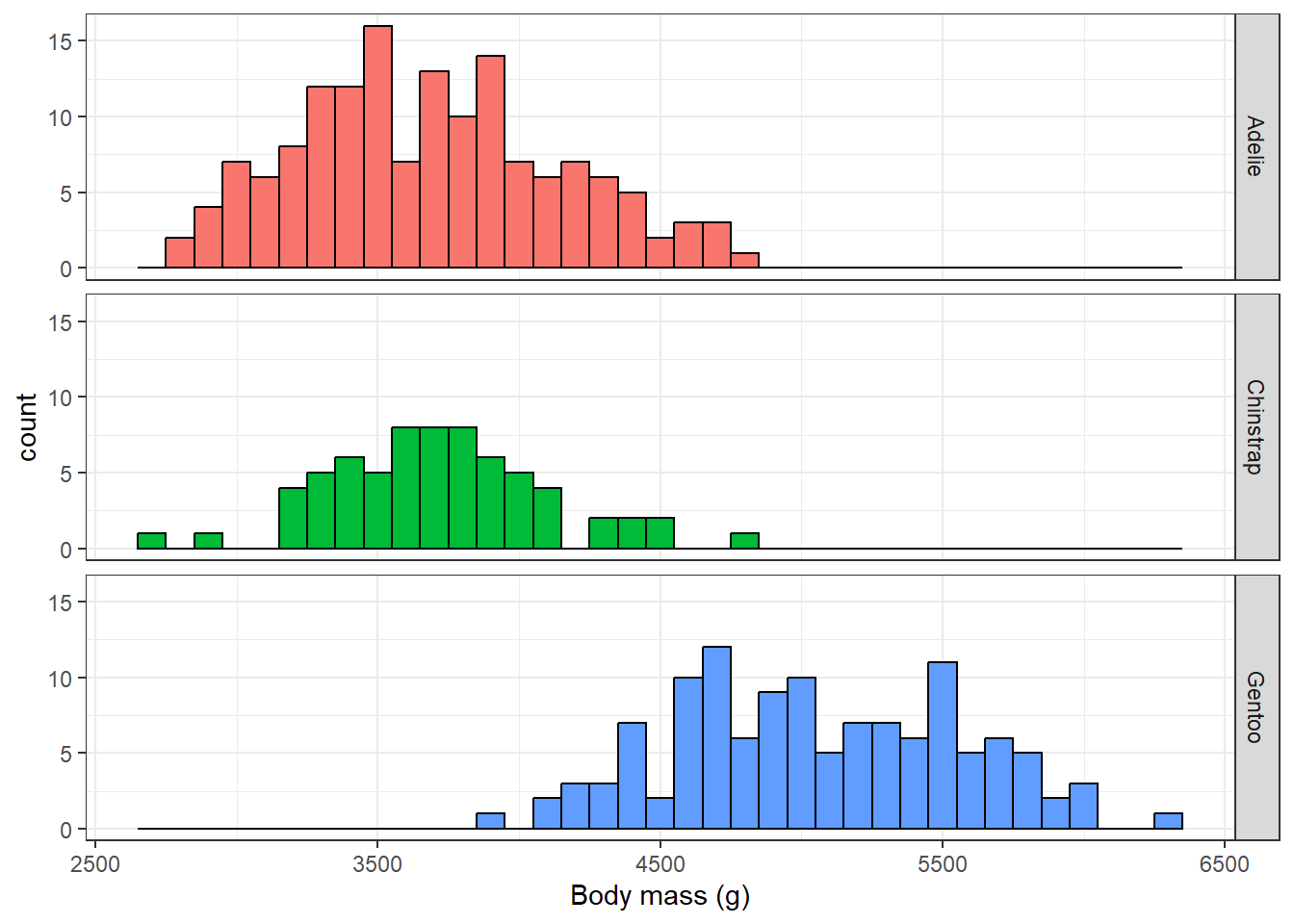
Choosing the right time to collect
collect() brings data out of the database and into R. Above we use it to bring the entire penguins data back into R so that we can then use ggplot() to make our histogram.
When working with large data sets, as is often the case when interacting with a database, we typically want to keep as much computation as possible on the database side, up until the point we need to bring the data out for further analysis steps that are not possible using SQL. This could be like the case above for plotting, but could also be for other analytic steps like fitting statistical models. In such cases it is important that we only bring out the required data for this task as we will likely have much less memory available on our local computer than is available for the database.
Now let’s look at the relationship between body mass and bill depth.
penguins |>
  collect() |>
  ggplot(aes(x = bill_depth_mm, y = body_mass_g)) +
  geom_point() +
  geom_smooth(method = "lm", se = FALSE) +
  xlab("Bill depth (mm)") +
  ylab("Body mass (g)") +
  theme_bw() +
  theme(legend.position = "none")
Here we see a negative correlation between body mass and bill depth which seems rather unexpected. But what about if we stratify this query by species?
penguins |>
  collect() |>
  ggplot(aes(x = bill_depth_mm, y = body_mass_g)) +
  facet_grid(species ~ .) +
  geom_point() +
  geom_smooth(method = "lm", se = FALSE) +
  xlab("Bill depth (mm)") +
  ylab("Body mass (g)") +
  theme_bw() +
  theme(legend.position = "none")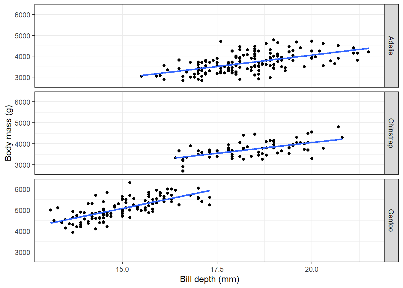
As well as having an example of working with data in database from R, you also have an example of Simpson´s paradox!
1.7 Disconnecting from the database
And now we’ve reached the end of this example, we can close our connection to the database.
dbDisconnect(db)